Skip to content

Amazon Redshift is a cloud data warehouse built for analytics at scale. It’s a common choice for teams running BI, reporting, and data transformation on AWS.
Redshift is also frequently positioned as a cost-effective alternative to platforms like Snowflake and BigQuery. But is that true?
This guide explains how Redshift pricing really works, how it stacks up, and gives you a practical optimization playbook you can apply like a pro.
What Is Amazon Redshift
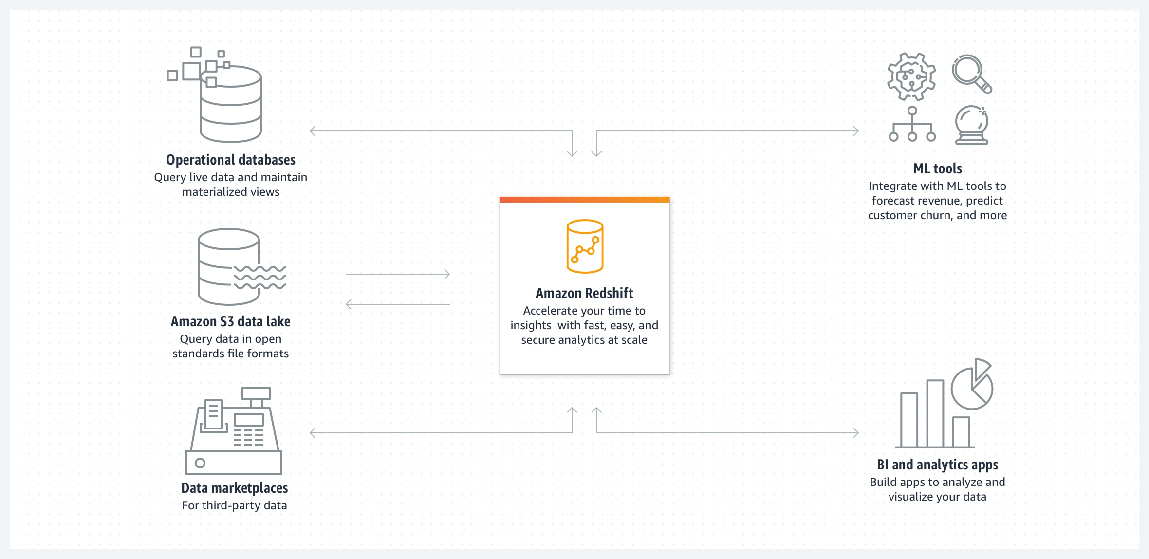
Amazon Redshift is AWS’s managed data warehouse for analytics: you load structured/semi-structured data into it (or query it in S3), then run standard SQL to power dashboards, reporting, and large-scale aggregations. Under the hood it’s built for analytical workloads using a distributed, columnar architecture (MPP) so it can scan and aggregate large tables efficiently compared to a traditional OLTP database.
How Redshift Pricing Works
Amazon Redshift costs vary based on factors like your AWS Region and how you run the service (cluster type/size and how long it runs).
In general, Redshift pricing falls into a few main models—on-demand, reserved/committed discounts, and serverless usage-based pricing—plus add-ons like storage, data transfer, and features such as Spectrum.
Provisioned clusters
With provisioned Redshift, you run an Amazon Redshift cluster of fixed capacity that you size up front. You choose a node type (family) and a node count, and you’re billed for compute costs while the cluster is running. This is the “classic” Redshift operating model: predictable capacity, predictable performance envelope, and cost that tracks how long you keep the cluster online.
Two details matter early for understanding the bill. First, your AWS Region and node type drive the baseline rate. If you enable Multi-AZ for a provisioned cluster, compute charges effectively double because the cluster runs in two AZs. Second, newer RA3 nodes separate compute from storage, which means scaling decisions can be more intentional: you’re not forced to pay for extra local SSD just to get more CPU/memory, and storage growth shows up as its own line item (Redshift Managed Storage) rather than being bundled into the node price.
Provisioned clusters also give you lifecycle controls. If the warehouse only needs to be available during business hours or batch windows, you can pause/resume to stop compute charges while keeping data persisted (you still pay storage).
On Demand vs Reserved Instances
For provisioned clusters, the difference between On-Demand pricing and Reserved pricing is mostly about commitment.
On-Demand is pay-as-you-go. You don’t commit to a term or pay up front; you’re charged for the provisioned compute capacity while it’s running, and billing is granular (per-second for partial hours). This is the most flexible option: you can change node types, resize, and pause/resume as your needs shift. When you pause a cluster, on-demand compute billing stops, but storage still applies.
Reserved Instances (Reserved Nodes) are for steady baselines. You commit to a term (typically 1 or 3 years) for specific node attributes in a specific Region in exchange for discounted pricing. Operationally, you’re not “creating nodes” when you buy a reservation—you’re purchasing a pricing commitment that applies to matching running capacity. This is why reservations are powerful when your footprint is stable, and frustrating when your footprint changes.
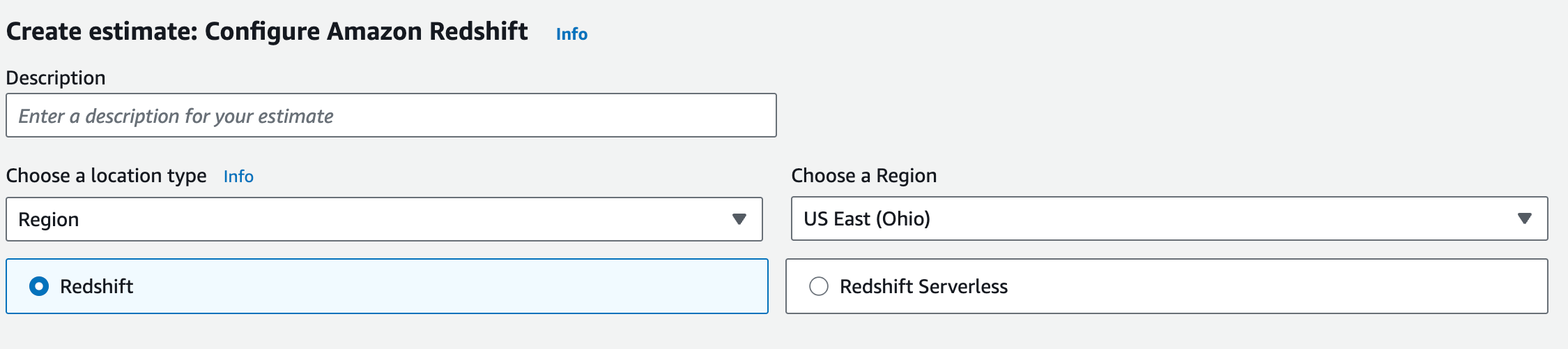
Redshift Serverless
Redshift Serverless changes the unit you pay for. You don’t size nodes or manage a cluster; instead, Redshift charges for compute based on RPU-hours. Usage is metered per-second, with a minimum charge window, and you can set bounds (like base/max capacity) to control spend and query performance behavior. Serverless lets you control spend and performance with Base (baseline RPUs), Max (usage limit in RPU-hours), and MaxRPU (cap on scaling).
The practical implication is simple: serverless fits teams that don’t want a warehouse running all the time, or workloads that are naturally bursty—where paying for always-on provisioned capacity would be wasteful. It can also reduce the operational overhead of resizing and capacity planning.
One important pricing nuance: in serverless, Concurrency Scaling and Spectrum are included in the RPU-based pricing, rather than billed as separate feature line items the way they can be with provisioned clusters.
Producer–consumer and multi-warehouse patterns
Once Redshift supports multiple workloads, pricing stops being just “how big is the warehouse?” and becomes “how many warehouses, for whom, and when?”
A common enterprise pattern is producer–consumer: one “producer” warehouse (or pipeline) prepares and publishes datasets, while separate “consumer” warehouses serve BI, ad hoc analysis, or data science. This can be advantageous from a cost point of view because instead of scaling one shared warehouse to satisfy the noisiest peak, you isolate capacity so each workload can scale (and be governed) on its own terms.
Redshift data sharing enables this model by letting multiple warehouses access the same data without copying it, which can reduce duplication and simplify governance. The tradeoff is that the easier you make it for consumers to query, the more likely overall query volume grows—so this pattern works best when ownership and guardrails are clear.
What Determines Your Redshift Cost
Here are the most important cost drivers of your overall bill. Let’s summarize:
| Cost driver | What it measures | What typically makes it rise |
|---|---|---|
| Compute | Capacity × time (nodes/RPUs running) | Always-on runtime, peak provisioning, more concurrent users/workloads |
| Storage | Data retained in Redshift-managed storage | Data growth, duplicated datasets/environments, retention that never shrinks |
| Query execution | Work required per query | Wide scans, frequent BI refreshes/scheduled runs, expensive joins/sorts |
| Backups & snapshots | Snapshot/backup footprint over time | Manual snapshot sprawl, long retention defaults, cross-region copies |
| Data transfer & consumption | Data moved to where it’s used | Cross-region consumers, frequent unload/exports, repeated downstream pulls |
| Managed storage (RMS) | Data stored in Redshift Managed Storage | Data retained in RA3/Serverless, retention policies |
| Concurrency scaling / burst | Extra compute during concurrency spikes | Queueing/high concurrency on provisioned clusters (beyond free credits) |
| Features | Metered feature usage beyond base compute/storage | Spectrum scan volume, concurrency-related usage, etc. |
Practical tips for Redshift Cost Optimization
Having discussed how pricing and billing work, let’s dive into a few cost savings and performance optimization tips — through better query patterns and more efficient use of compute resources.
1. Right-Size Compute
Right-sizing starts with one step: identify what’s forcing you to buy more capacity—CPU, memory, concurrency, or I/O—because each points to a different fix. CPU pressure looks like slow scans/aggregations even at low concurrency; memory pressure shows up when complex joins/sorts degrade as data grows; concurrency pressure shows up as queueing; and I/O pressure shows up as disproportionate time spent moving data.
Once you know the constraint, size for the normal day and handle the peak deliberately. For predictable spikes, use scheduled scaling; for mixed workloads that collide, separate them so one peak doesn’t dictate capacity for everyone. If the workload is intermittent, don’t run capacity just in case—pause/schedule low-duty warehouses. And if you’re on RA3, treat compute and storage as separate decisions: don’t scale compute just because data grows.
2. Use WLM and QMR to Prevent Expensive Queries
Since Redshift performance depends heavily on how much data each query reads and how workloads share resources, the fastest path to lower cost is often to improve query performance.
WLM determines how work is prioritized when the warehouse is busy, and QMR lets you automatically constrain queries that would otherwise consume disproportionate resources. The goal is to prevent two common cost outcomes: BI latency getting dragged down by batch workloads, and runaway queries forcing you to increase baseline capacity to compensate.
Keep it simple: create separate WLM queues for interactive and batch, and make the default queue conservative so ad hoc usage does not get unlimited runway. Then add a small set of QMR guardrails that cancel or reroute queries when they exceed clear boundaries such as runtime, spill volume, or scan thresholds. Done well, WLM and QMR reduce cost by keeping bad workloads from becoming the reason you resize.
3. Keep Storage Lean With Retention and Data Lifecycle Management
Storage cost usually creeps up because data rarely gets deleted by accident, but it often gets retained by default. The practical move is to define retention rules by dataset class, then enforce them so raw and intermediate data does not accumulate indefinitely while curated datasets stay stable and trusted.
Tiering is the second lever: keep frequently queried, latency-sensitive data in Redshift, and push cold history to cheaper storage with a clear access path for occasional analysis. This keeps the warehouse from becoming the long-term archive for everything and prevents storage growth from silently turning into compute growth later when larger tables become the default scan target.
4. Reduce Query Cost by Cutting Scanned Bytes
From there, prioritize changes that reduce read data volume, and that you can validate quickly. Start by narrowing the columns each query touches to only what the result actually uses, because wide selects quietly multiply I/O on every refresh and rerun. Then make filtering patterns consistent across the tools generating the workload so the engine can reliably prune what it does not need to read. Finally, make the time window explicit for recurring queries so you are not scanning full history when the dashboard only needs recent periods. After each change, re-run the same query and confirm bytes scanned dropped; that metric is the clearest signal you made the workload cheaper at scale and not just different.
5. Make Loads Cheaper With Batch and Incremental Patterns
Redshift load costs usually spike for two reasons: you are loading too often in small chunks, or you are reprocessing more data than the business change actually requires. The practical default is to batch work into fewer, larger runs and make transformations incremental so each run only touches new or changed data.
At the pipeline level, this means sizing files and batches so loads are efficient, and designing jobs so reruns do not automatically trigger full reloads of historical partitions. For transformation workloads, favor models that update the smallest possible slice of data each run, and treat large backfills as planned events with explicit scope instead of routine behavior.
6. Use Spectrum Deliberately
Redshift Spectrum is most effective when it has a clear job: keep infrequently accessed or long-tail history in S3 and query it only when needed, while keeping high-traffic, latency-sensitive datasets inside Redshift. Costs rise when Spectrum becomes the default path for broad, repeated scans, especially from BI tools and scheduled jobs, because spend tracks how much data you read. The practical approach is to decide which datasets are meant to be queried externally, organize them so typical queries touch a small slice, and put simple governance around who can run large scans and how often.
7. Control Snapshots and DR Footprint
Snapshot and DR (Disaster Recovery) retention costs grow when defaults become permanent and manual snapshots pile up without an expiry. The fastest way to get this under control is to treat snapshots like any other asset: every snapshot should have an owner, a purpose, and a deletion date.
Set retention targets by environment and criticality, since production, staging, and development should not carry the same recovery footprint. Then enforce lifecycle discipline: require manual snapshots to include an expiry in the name or tags, review snapshot inventory on a cadence, and restrict cross-region copies to the minimum set required by your DR plan.
8. nOps for Amazon Redshift Cost Efficiency
nOps is a cloud cost optimization platform that helps you understand, control, and reduce Amazon Redshift spend with no manual effort.
Visibility into Redshift cost drivers
nOps breaks Redshift spend down into any useful engineering or finance dimension—such as by account, environment, team, application, and region—so you can quickly answer: Which cluster or workgroup changed? What changed about it? And what should we do next? It also includes cost anomaly detection, forecasting, budgeting, reporting, and all the other features you need.
Cost allocation that makes ownership obvious
nOps automates tagging and cost allocation, so you can break down spending by team, customer, product, or any other cost center.
Autonomous commitment management savings
If you’re running Redshift at any real scale, nOps takes commitments off your plate. It automatically selects the right AWS commitment approach for your Redshift usage and keeps it aligned as your footprint changes—so you capture savings without spending time modeling options, purchasing plans, or continually rebalancing coverage.
Want to see it in practice? Book a demo to walk through Redshift cost visibility, allocation, and spike protection in your environment.
nOps manages $3 billion in AWS spend and was recently rated #1 in G2’s Cloud Cost Management category.
Frequently Asked Questions
Let’s briefly address a few FAQ relating to Amazon Redshift.
What are the biggest factors that impact Amazon Redshift cost and performance?
Data movement, actual usage patterns, loading data, and data encryption all influence Redshift spend and query speed in different ways: data movement increases work during joins and reshuffles, actual usage patterns determine whether you’re paying for steady baselines or peaks, loading data inefficiencies can multiply runtime and retries, and data encryption adds necessary security controls that can affect overhead and design decisions depending on how you implement it.
How can data analysts improve performance on large datasets in Redshift Serverless while keeping operating costs predictable?
Query complexity and data scanned are usually the biggest levers for Redshift Serverless spend because Redshift Processing Units scale with actual work done, so reducing unnecessary scans helps keep predictable costs. Using data compression and sensible data management for historical data can also reduce storage costs and keep dynamic workloads from getting slower as tables grow. To allocate resources efficiently, set clear workload boundaries and controls so bursty, specific workloads don’t consume more Processing Units than they need.